|
3.4 The Elliptical Structure Theorem
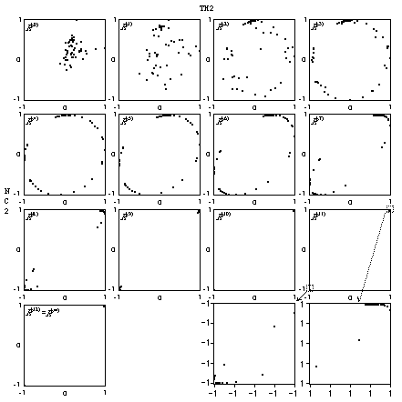
For another picture of convergence, two variables were randomly selected from the fifty symptoms and their scatterplots were displayed at each iteration. The sequence of scatterplots for columns TH2 and NC2 are displayed in Figure 5. An interesting pattern of a gradually formed ellipse is identified in the sequence of the
scatterplots. The near perfect ellipse was formed at matrices  to
to  and later these fifty points rapidly converge to the points (1, 1) and (-1, -1). These two point clusters are then magnified at matrix and later these fifty points rapidly converge to the points (1, 1) and (-1, -1). These two point clusters are then magnified at matrix
 , one iteration from , one iteration from  , and similar elliptical structure in these two epsilon boxes was identified. The point-clouds concentrate on the lower left and upper right corners indicating that these two columns (symptoms) converge to the same group. , and similar elliptical structure in these two epsilon boxes was identified. The point-clouds concentrate on the lower left and upper right corners indicating that these two columns (symptoms) converge to the same group.

Figure 5. Sequence of Scatterplots of Symptoms TH2 and NC2.
Actually, this formation of ellipse in the scatterplot for the correlation matrices exists in all C(50, 2) = 1225 possible pairs of columns. The following theorem and corollaries say that every correlation matrix
 in the converging sequence has it's column vectors fall on the surface of the in the converging sequence has it's column vectors fall on the surface of the
 -dimensional ellipsoid generated by the kernel -dimensional ellipsoid generated by the kernel
 or or  , the inverse or generalized inverse of , the inverse or generalized inverse of
 . .
Theorem 3.1.
Given a full rank correlation matrix R, all p column (row) vectors of R,
 , i=1,…,p, fall on the p-dimensional ellipsoid generated by the kernel of , i=1,…,p, fall on the p-dimensional ellipsoid generated by the kernel of
 , the inverse of R. , the inverse of R.
Proof. Observe that the right hand side of the equality
 is a correlation matrix, hence all diagonal elements equal one. That is
diag( is a correlation matrix, hence all diagonal elements equal one. That is
diag( ) = diag( ) = diag( ) =(1,1,…,1), which leads to ) =(1,1,…,1), which leads to
 , i=1,…,p, thus completing the proof. , i=1,…,p, thus completing the proof.
In general, only the original proximity matrix D could be of full rank, all the subsequent correlation matrices
 have ranks smaller than p, the dimension of D. We can then substitute have ranks smaller than p, the dimension of D. We can then substitute
 in Theorem 3.1 with the generalized inverse in Theorem 3.1 with the generalized inverse
 . When the correlation matrix is not orthogonal, usually the case, we have a rotated version of Theorem 3.1. . When the correlation matrix is not orthogonal, usually the case, we have a rotated version of Theorem 3.1.
Corollary 3.1.
Given a p-dimensional correlation matrix  with rank
  , and the spectral decomposition , and the spectral decomposition
 , where , where  is a k-dimensional diagonal matrix with a list of non-zero eigenvalues (
 , , ,…, ,…, ) ( ) ( are not necessarily distinct) on the diagonal and are not necessarily distinct) on the diagonal and
 contains the contains the  eigenvectors
  , , ,… ,… . All the p principal components of . All the p principal components of
 , ,  , i=1,…,p fall on the k-dimensional ellipsoid generated by the kernel of , i=1,…,p fall on the k-dimensional ellipsoid generated by the kernel of
 , the inverse of , the inverse of  . .
Usually when one deals with the ellipsoid generated from the quadratic form of a positive definite matrix like the correlation matrix, then it is Corollary 3.2 that is of interest and not Corollary 3.1.
Corollary 3.2. With the same setup as in Corollary 3.1, all the p rows of
 , ,  , i=1,…,p fall on the k-dimensional ellipsoid generated by the kernel of , i=1,…,p fall on the k-dimensional ellipsoid generated by the kernel of
 . .
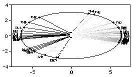
Figure 6 shows these two ellipse generated by
 and and  for the fifty columns at
  with all the fifty with all the fifty
 ’s and ’s and  ’s falling on them. Besides, the half-lengths of the principal axes for these two ellipsoids can be computed from the
eigenvalues. For the ellipsoid generated by ’s falling on them. Besides, the half-lengths of the principal axes for these two ellipsoids can be computed from the
eigenvalues. For the ellipsoid generated by  , we have , we have
[  … …
 ]diag[ ]diag[  … …
 ][ ][  … …
 ]T=1, so ]T=1, so  =1. =1.
The half-length for each principal axis of the ellipsoid generated by
 is is  , i=1,…,k. For the ellipsoid generated by , i=1,…,k. For the ellipsoid generated by
 , the half-lengths are , the half-lengths are  , i=1,…,k. In Figure 6, these half-lengths are (6.401851, 3.002717) for , i=1,…,k. In Figure 6, these half-lengths are (6.401851, 3.002717) for
 and (0.156205, 0.333032) for and (0.156205, 0.333032) for  . .

Figure 6. Two Ellipses Generated by
 (outer) and (outer) and  (inner) for the Fifty Symptom Example.
We have now shown that each of the correlation matrix in the sequence
 has an exact has an exact  -dimensional ellipsoid structure embedded in it. In the converging process, each time the rank (numerical) decreases, the ellipsoid collapses down to a lower dimensional one. The sequence of scatterplots for symptoms TH2 and NC2 with elliptical structure in Figure 5 are the two-dimensional images projected from the fifty-dimensional ellipsoids. The plotting of leading eigenvectors with ellipses to study the structure of original proximity matrix D is illustrated in Section 5.1. -dimensional ellipsoid structure embedded in it. In the converging process, each time the rank (numerical) decreases, the ellipsoid collapses down to a lower dimensional one. The sequence of scatterplots for symptoms TH2 and NC2 with elliptical structure in Figure 5 are the two-dimensional images projected from the fifty-dimensional ellipsoids. The plotting of leading eigenvectors with ellipses to study the structure of original proximity matrix D is illustrated in Section 5.1.
|