The concept of using points of different shading to represent proximity measurements is not at all new to researchers in the fields of gene expression (Vishwanath et al. (1999), Wen et al. (1998)), taxonomy (Sneath and Sokal (1973)), seriation (Caraux (1984), Streng (1991)), cluster analysis (Gale and Halperin (1984), Streng (1991)), statistical computing (Murdoch and Chow (1996)) and multidimensional scaling (Chen and Chen (1998)).

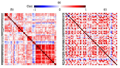
Constructing a proximity matrix map is illustrated here using the Pearson product-moment correlation matrix of the fifty symptoms (Kendall's rank correlation and other possible association measurements produce similar result). Given a proximity matrix (correlation in this case), first a color spectrum is selected, suitable for representing the range and scale for the measurements of the proximity matrix. For the correlation matrix, the blue-red spectrum is shown in Figure 2a. The whole proximity matrix is then projected through the color spectrum to get the color proximity matrix map as shown in Figure 2b. From Figure 2b the blocks of dark red points on the main diagonal can be easily located. Thirty positive symptoms are divided into several small groups of symptoms; whereas, all the twenty negative symptoms form a more coherent cluster except symptoms NE1 and NE2 on the lower right corner.

Murdoch and Chow (1996) cleverly used elliptical glyphs to represent correlations. However, their method is for displaying only correlation matrices and not for other types of proximities.

Figure 2. The Colored Correlation Matrix Maps for the Fifty Symptoms.(a). Blue-Red Color Spectrum for Correlation Coefficients;  (b). Correlation Matrix Map with the Original SAPS/SANS Order;  (c). Correlation Matrix Map with a Random Permutation.

The Seriation Problem

From Figure 2b, the grouping effect of variables and the structure between the groups can be easily retrieved. However, this is not always true for proximity matrix maps. When the fifty symptom’s correlation map was constructed, the variables were laid out in a prespecified order from the Andreasen’s symptom scale table. The symptoms are listed in groups hence we see the blocks on the main diagonal in Figure 2b. These fifty symptoms are grouped in advance since the researchers have already done a detailed analysis on them. We do not always have the variables grouped in advance, especially before initial data analysis. Therefore, to find out the changes on the correlation map if the variables are listed in a random manner the fifty symptoms were randomly permuted and the correlation map reconstructed as shown in Figure 2c. A dramatic change is observed from Figure 2b to that in Figure 2c. Almost everything is lost: the structured patterns, the blocks, and the relationship between the groups. All information (correlation coefficients) from the original proximity matrix was kept while the map was reconstructed but the pattern has disappeared.

In order to recover the missing structure from Figure 2c, or even to get a better structure than Figure 2b, we need a seriation algorithm. Seriation is a data analytic tool for finding a permutation or ordering of a set of objects using a data matrix (symmetric or asymmetric). In the 19th century, archaeologists and prehistory researchers used seriation as a dating technique for ancient objects using certain attributes for description. In an early survey, Hubert (1976) conducted an interesting study of seriation problems from various research fields with their different names and computational approaches. In a more recent survey, Marcotorchino (1991) discussed the seriation problem from the aspect of problem setting, methodology and algorithms.

Using Marcotorchino’s (1991) notation, the initial matrix is denoted as T, with the set of objects and the set of variables denoted as I and J respectively. The basic principle of seriation is to find a reshaped matrix T’ with a permutation of I, together with a permutation of J, to identify the embedded latent structure. When T is symmetric, we usually want T’ to approximate a Robinson form (Robinson (1951)). (A matrix T is said to be a Robinson matrix if the elements in its rows and columns do not increase when moving horizontally or vertically away from the main diagonal.

Reference: